Operating System

Outline

Architecture

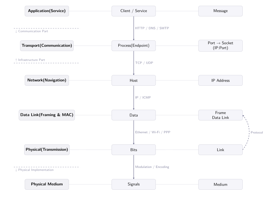
In OSI, the Presentation Layer and Session Layer are implemented in the Application Layer.
In TCP/IP, the Network Access Layer is implemented in the Data Link Layer and Physical Layer.

Philosophy

Logical Architecture v.s. Physical Implementation: Transparency
Efficiency v.s. Reliability: Multiplexing
OSI v.s. TCP/IP: Error Handling and Synchronization

Physical Layer

The Sampling Theorem*

The Nyquist-Shannon Sampling Theorem is the foundation of all digital communication. It states:

A continuous-time signal $s(t)$ that is strictly bandlimited to $B$ Hz (i.e., its Fourier transform $S(f) = 0$ for $|f| > B$) can be perfectly reconstructed from its discrete samples $s(nT_s)$, provided the sampling rate satisfies $f_s = 1 / T_s \ge 2B$.

Let $s(t)$ be a bandlimited signal with $S(f) = 0$ for $|f| > B$. Sampling at intervals $T_s = 1/f_s$ can be modeled as multiplication by a Dirac comb:

$$ s_{\text{sampled}}(t) = s(t) \cdot \sum_{n=-\infty}^{\infty} \delta(t - nT_s) $$

Taking the Fourier transform and using the convolution theorem, the spectrum of the sampled signal is:

$$ S_{\text{sampled}}(f) = S(f) * \mathcal{F}\!\left\{\sum_{n} \delta(t - nT_s)\right\} = S(f) * \left( f_s \sum_{k=-\infty}^{\infty} \delta(f - k f_s) \right) = f_s \sum_{k=-\infty}^{\infty} S(f - k f_s) $$

This reveals that sampling replicates the original spectrum at integer multiples of $f_s$.

Now consider two cases:

$f_s \ge 2B$ (no aliasing). The replicas $S(f - k f_s)$ are separated by $f_s \ge 2B$, so adjacent copies do not overlap. An ideal low-pass filter

$$ H(f) = \begin{cases} \frac{1}{f_s}, & |f| \le B \\\\ 0, & |f| > B \end{cases} $$

extracts $S(f)$ exactly: $S_{\text{sampled}}(f) \cdot H(f) = S(f)$. Taking the inverse Fourier transform yields the Whittaker-Shannon interpolation:

$$ s(t) = \sum_{n=-\infty}^{\infty} s(nT_s) \cdot \operatorname{sinc}\!\left(\frac{t - nT_s}{T_s}\right), \qquad \operatorname{sinc}(x) = \frac{\sin(\pi x)}{\pi x} $$

$f_s < 2B$ (aliasing). The replicas overlap — high-frequency components from $S(f - f_s)$ fold into the baseband $[-B, B]$, corrupting $S(f)$. No filter can separate them; the original signal is irrecoverably distorted. This is why the critical rate $f_{\text{Nyquist}} = 2B$ is the minimum sampling rate for perfect reconstruction.

Nyquist Theorem*

The Nyquist theorem applies the Sampling Theorem to data communication: it gives the maximum symbol rate over a noiseless low-pass channel of bandwidth $B$ Hz. If each symbol carries $\log_2 V$ bits (i.e., $V$ discrete signal levels), the maximum data rate is:

$$ C_{\text{noiseless}} = 2B \cdot \log_2 V \quad \text{(bps)} $$

Proof (via the Sampling Theorem).

A signal $s(t)$ strictly bandlimited to $B$ Hz can be perfectly reconstructed from its samples taken at rate $f_s \ge 2B$:

$$ s(t) = \sum_{n=-\infty}^{\infty} s\!\left(\frac{n}{2B}\right) \cdot \operatorname{sinc}\!\big(2Bt - n\big) $$

where $\operatorname{sinc}(x) = \frac{\sin(\pi x)}{\pi x}$. This means that all information in a bandlimited signal of duration $T$ is captured by $2BT$ independent samples — one every $\frac{1}{2B}$ seconds. If we treat each sample as a transmitted symbol, the maximum symbol rate is $2B$ baud. With $V$ discrete levels per symbol, each carries $\log_2 V$ bits, yielding the formula above.

Key takeaways:

For binary signals ($V = 2$), the maximum rate is $2B$ bps — exactly twice the bandwidth.
To increase the data rate, one can increase either the bandwidth $B$ or the number of levels $V$. However, $V$ cannot grow arbitrarily — more levels mean smaller gaps between adjacent levels, making the signal more vulnerable to noise. This is where the Shannon theorem comes in.

Intuition: Nyquist tells us the maximum number of distinguishable symbols per second in a perfect, noise-free world. It bounds the symbol rate ($2B$ baud), not the bit rate — the bit rate depends on how many bits each symbol encodes.

Shannon Theorem*

The Shannon-Hartley theorem extends Nyquist by incorporating noise, giving the theoretical upper bound for reliable communication over a noisy channel:

$$ C = B \cdot \log_2 (1 + \text{SNR}) \quad \text{(bps)} $$

where $\text{SNR}$ is the signal-to-noise ratio (linear), typically given in decibels (dB):

$$ \text{SNR}_{\text{dB}} = 10 \cdot \log_{10} \left( \frac{P_{\text{signal}}}{P_{\text{noise}}} \right) \quad \Rightarrow \quad \text{SNR}_{\text{linear}} = 10^{\text{SNR}_{\text{dB}} / 10} $$

Proof (sketch for the AWGN channel).

Consider a discrete-time additive white Gaussian noise (AWGN) channel:

$$ Y = X + N, \qquad N \sim \mathcal{N}(0, \sigma^2) $$

with a power constraint $\mathbb{E}[X^2] \le P$. The channel capacity is defined as the maximum mutual information over all input distributions satisfying the constraint:

$$ C = \max_{p(x):\; \mathbb{E}[X^2] \le P} I(X; Y) $$

Expand the mutual information using differential entropy:

$$ I(X; Y) = h(Y) - h(Y \mid X) = h(Y) - h(N) \tag{1} $$

where $h(Y \mid X) = h(N)$ because $N$ is independent of $X$. The differential entropy of a Gaussian with variance $\sigma^2$ is:

$$ h(N) = \frac{1}{2} \log_2\!(2\pi e \sigma^2) \tag{2} $$

For $Y = X + N$, its variance is $\operatorname{Var}(Y) = P + \sigma^2$ (since $X$ and $N$ are independent). Among all distributions with a given variance, the Gaussian maximizes differential entropy. Hence:

$$ h(Y) \le \frac{1}{2} \log_2\!\big(2\pi e (P + \sigma^2)\big) \tag{3} $$

with equality when $Y$ is Gaussian — which occurs when $X \sim \mathcal{N}(0, P)$. Substituting (2) and (3) into (1):

$$ I(X; Y) \le \frac{1}{2} \log_2\!\left(1 + \frac{P}{\sigma^2}\right) \quad \text{bits per channel use} $$

By the Nyquist sampling theorem, a bandlimited channel of bandwidth $B$ supports $2B$ independent channel uses per second. Multiplying by $2B$:

$$ C = B \cdot \log_2\!\left(1 + \frac{P}{\sigma^2}\right) = B \cdot \log_2\!(1 + \text{SNR}) $$

Key implications:

$C$ is a hard upper bound: there exists some coding scheme that can approach this rate arbitrarily closely with vanishingly small error probability, but it can never be exceeded.
Bandwidth and SNR are interchangeable: for a given capacity $C$, one can trade a wider bandwidth for a lower SNR (the principle behind spread-spectrum communication), and vice versa.
As $B \to \infty$, $C \to 1.44 \cdot (P_{\text{signal}} / N_0)$, showing that even with infinite bandwidth, capacity is still capped by the ratio of signal power to noise power spectral density.

Nyquist tells us how many symbols we need; Shannon tells us how much information those symbols can carry in the presence of noise. Together, they define the fundamental limits of any physical channel.

Modulation and Coding

Data Link Layer

implement:

Architecture

Layer	Role	2
	数据2	数据3
数据4	数据5	数据6
数据4	数据5	数据6
数据4	数据5	数据6
Data Link		数据6
Physical	数据5	数据6

$$\text{?}\xrightarrow{\text{Modulation}}\text{Frame}\xrightarrow{\text{Coding}}\text{Signal}$$

Operating System

Outline

Architecture

Philosophy

Physical Layer

The Sampling Theorem*

Nyquist Theorem*

Shannon Theorem*

Modulation and Coding

Data Link Layer

Architecture

Error Control

MAC

CDMA

真令牌

自学习算法

STP 生成树协议 STA

ICMP & Ping

References

Outline#

Architecture#

Philosophy#

Physical Layer#

The Sampling Theorem*#

Nyquist Theorem*#

Shannon Theorem*#

Modulation and Coding#

Data Link Layer#

Architecture#

Error Control#

MAC#

CDMA#

真令牌#

自学习算法#

STP 生成树协议 STA#

ICMP & Ping#

References#

Outline

Architecture

Philosophy

Physical Layer

The Sampling Theorem*

Nyquist Theorem*

Shannon Theorem*

Modulation and Coding

Data Link Layer

Architecture

Error Control

MAC

CDMA

真令牌

自学习算法

STP 生成树协议 STA

ICMP & Ping

References

- 2027年计算机网络考研复习指导,王道论坛。